構造化照明顕微鏡法(SIM)画像を使用した時空間画像相関スペクトル法により、T細胞の皮質アクチン流動を定量化
Abstract
Filamentous-actin plays a crucial role in a majority of cell processes including motility and, in immune cells, the formation of a key cell-cell interaction known as the immunological synapse. F-actin is also speculated to play a role in regulating molecular distributions at the membrane of cells including sub-membranous vesicle dynamics and protein clustering. While standard light microscope techniques allow generalized and diffraction-limited observations to be made, many cellular and molecular events including clustering and molecular flow occur in populations at length-scales far below the resolving power of standard light microscopy By combining total internal reflection fluorescence with the super resolution imaging method structured illumination microscopy, the two-dimensional molecular flow of F-actin at the immune synapse of T cells was recorded. Spatio-temporal image correlation spectroscopy (STICS) was then applied, which generates quantifiable results in the form of velocity histograms and vector maps representing flow directionality and magnitude. This protocol describes the combination of super-resolution imaging and STICS techniques to generate flow vectors at sub-diffraction levels of detail. This technique was used to confirm an actin flow that is symmetrically retrograde and centripetal throughout the periphery of T cells upon synapse formation.
Introduction
The goal of the experiment is to image and characterize the molecular flow of filamentous- (F-) actin in living T cells, beyond the diffraction limit in order to establish flow direction and magnitude during immunological synapse (IS) formation. This technique will be carried out using a structured illumination microscope (SIM) in total internal reflection fluorescence (TIRF) mode, imaging Jurkat T-cells forming an artificial synapse on activating coverslips coated with anti-CD3- and anti-CD28 antibodies. The IS forms between a T cell and its target; an antigen presenting cell (APC) upon T cell receptor (TCR) activation1,2. As this is the first step in determining whether the adaptive immune system generates an immune response to an infection, the consequences of incorrect responsiveness to stimuli can cause a number of diseases. The importance of the T cell-APC interaction is well documented, however, the role(s) of the mature IS after initial TCR signal internalization are yet to be fully understood.
As the cytoskeleton is thought to aid two processes linked to TCR activation (the movement of molecules at the plasma membrane and the control of signaling molecules dependent on the actin cytoskeleton3,4 ), understanding how the cytoskeleton rearranges spatially and temporally will elucidate the steps of molecular reorganization during synapse formation. The retrograde flow of F-actin is thought to corral TCR clusters towards the center of the immunological synapse, this translocation is believed to be vital for signal cessation and recycling; aiding the fine balance of T cell activation5.
While standard fluorescence microscopy is a flexible tool that continues to provide insight about many biological events including cell-cell interactions, it is limited by the system's ability to accurately resolve multiple fluorophores residing closer than the diffraction limit (≈200 nm) of each other. As many molecular events within cells involve dense populations of molecules and exhibit dynamic rearrangement either in quiescence or upon specific stimulation, conventional light microscopy does not provide the full picture.
The use of super resolution imaging has allowed researchers to circumvent the diffraction limit using a variety of techniques. Single molecule localization microscopy (SMLM) such as PALM and STORM6,7 has the ability to resolve the location of molecules up to a precision of around 20 nm, however, these techniques rely on long acquisition times, building up an image over many frames. Generally this requires samples to be fixed or for structures to exhibit low mobility so single fluorophores are not misinterpreted as multiple points. While stimulated emission depletion (STED) imaging allows super-resolution through very selective confocal excitation8, the required scanning approach can be slow over whole cell fields of view. STED also demonstrates significant phototoxicity for higher resolutions due to the increase in power of the depletion beam.
Structured illumination microscopy (SIM9) provides an alternative to these methods, capable of doubling the resolution of a standard fluorescence microscope and is more compatible with live cell imaging than current SMLM techniques. It uses lower laser powers, on a wide-field system for whole-cell fields of view; providing increased acquisition speeds, and is compatible with standard fluorophore labelling. The wide-field nature of SIM also permits the utilization of total internal reflection fluorescence (TIRF) for highly selective excitation, with penetration depths in the axial dimension of <100 nm.
Image correlation spectroscopy (ICS) is a method of correlating fluctuations in fluorescence intensity. An evolution of ICS; Spatio-temporal image correlation spectroscopy (STICS10) correlates intracellular fluorescent signals in time and space. By correlating pixel intensities with surrounding pixels in lagging frames via a correlation function, information is gained regarding flow speeds and directionality. To ensure static objects do not interfere with the STICS analysis, an immobile object filter is implemented, which works by subtracting a moving average of the pixel intensities.
The technique presented here is believed to be the first demonstration of image correlation spectroscopy being applied to super-resolution microscopy data to quantify the molecular flow in live cells11. This method improves on diffraction-limited imaging of F-actin flow via STICS analysis12 and would suit researchers who wish to determine two-dimensional molecular flow in live cells, from data acquired at spatial resolutions beyond the diffraction limit of light.
Protocol
Note: Stages 1 and 2 take place before the day of imaging; ensure all media and supplements to be used before or on the day of imaging are equilibrated. Equilibration is achieved through warming of media and supplements to 37 °C in an incubator set to 5% CO2. All cell culture work and coverslip plating steps take place in sterile conditions under a laminar flow hood.
1. Cell Transfection
- Transfect the T cells to be imaged 24 hr before the experiment with a plasmid encoding a fluorescent fusion construct for F-actin GFP labelling and imaging. Note: Cells should be split 24 hr prior to transfection (48 hr prior to imaging) to ensure cells are at optimal health and in their logarithmic growth phase.
- Place 5 mL of RPMI supplement (RPMI 1640 plus 10% FBS and 1% Pen-Strep (optional)) in a single well of a 6-well plate into the incubator to equilibrate.
- Pellet 2 x 10⁷ T cells cultured at 37 °C +5 % CO2 in RPMI supplement using a centrifuge tube at 327 x g for 5 min and wash in an equal volume of pre-warmed electroporation media. Note: Electroporation medium is a reduced serum medium containing buffers and supplements (see consumables).
- After re-pelleting at 327 x g for 5 min, resuspend the cells in 500 µl of electroporation media and slowly add to a cuvette, add 5 µg of the plasmid in PCR grade dH2O for labelling F-actin.
- Gently tap the cuvette on the hood workspace to ensure removal of any air bubbles in the media, which can cause arcing of the electricity and to distribute the cells evenly within the media.
- Turn on the electroporation apparatus and set voltage to 300 V and capacitance to 290 Ω. Electroporate sample using an exponential decay for 20 msec. Note: Optimization may be required for different cells and different plasmid constructs.
- Once the transfection protocol is complete, store cells on ice for 1 min before continuing.
- Carefully transfer the cells from the cuvette to the 6-well plate containing 5 mL of equilibrated RPMI supplement from step 1.1.1.
- Incubate the cells O/N at 37 °C + 5% CO2.
2. Coat Coverslips and Pre-warm Imaging Supplement
- Coat coverslips with antibodies to induce T cell stimulation.
- Coat each chamber of an 8-well coverslip with 1 µg / ml αCD3 and αCD28 in 200 µl PBS.
- Store at 4 °C O/N. Alternatively, coat coverslips 2 hr prior to imaging and keep in an incubator at 37 °C to reduce drift during the imaging process by minimizing temperature changes to the coverslip.
- Create a coverslip test sample with 0.1 µm sub-diffraction fluorescent microspheres.
- Vortex stock solution of beads to avoid clumps.
- On a new, clean coverslip of the same type as those used in step 2.1.1, pipette 5 µl fluorescent microsphere stock solution onto the surface (as per manufacturer's instructions).
- Spread microsphere solution over the coverslip with pipette tip.
- Allow to dry, then apply 200 µl mounting medium such as PBS.
Note: the mounting medium should match that used for imaging cell samples.
- Equilibrate HBSS (+ 20 mM HEPES, hereafter called 'HBSS supplement') in a centrifuge tube by placing in an incubator to pre-warm O/N at 37 °C + 5% CO2.
Note: the addition of HEPES is to buffer CO2, if using an incubation chamber with CO2 input skip this supplementation.
3. Microscope Set-up
- Turn on the stage-top incubator of the TIRF-SIM microscope and place enough distilled water in the reservoir of the microscope to fully cover the base of the heating element. Allow water to equilibrate to 37 °C. Add the heating collar to the objective lens, also set to 37 °C.
Note: Due to the sensitivity of the set-up, these steps are done the night before so the optical components are at a stable temperature prior to imaging. - Place the TIRF 488 compatible grating block in the light path of the microscope and secure in place.
- Switch the channel mode and the fiber cable to the 'Single' position on the laser bed and microscope stage respectively to engage the correct optical path for the TIRF-SIM mode. Note: Skipping this step will lead to an error (Figure 1A) within the software window.
- Turn on all microscope and computer components and open the acquisition control software.
- Open the OC panel, Ti Pad, N-SIM Pad and ND Acquisition windows (Figure 1B). In the 'OC Panel' select the option 'TIRF 488' (Figure 2B, yellow arrow).
- In the N-SIM Pad window, select the 'TIRF-SIM' and 'Moving' settings (Figure 2C, yellow arrows). Select the settings button (Figure 1C, yellow box) and select 'TIRF 488 (for 100x TIRF 488nm)' from the dropdown menu, hit 'Apply' and 'OK'.
- Set the camera settings within the 'DU897 settings' to: Frame Rate 50 msec, Readout mode, EM Gain 3 MHz at 14-bit, and EM Gain Multiplier 300 with a Conversion Gain of 1 (Figure 1C, green box).
Note: see Representative Results for frame rate considerations. - Calibrate the microscope's illumination for TIRF-SIM by selecting the 100x 1.49 NA CFI Apochromat TIRF objective, on the 'N-SIM Pad' turn the 488 nm laser power to 10%.
Note: Pixel size of the raw images is 60 nm, with a 512 x 512 pixel field of view. - Clean the objective lens using lens tissue to remove dust and oil.
- Find the TIRF-SIM focal plane.
- Start with the objective in the lowest possible z-plane. Place a drop of lens oil on the objective and add the fluorescent microsphere sample from step 2.2 to the microscope stage.
- Select the Perfect Focus System (PFS) function located on the body of the microscope.
- Slowly move the objective up through the z-plane until the PFS button stops flashing to confirm the focal plane has been reached.
- Switch to 'Live' view on the control software and image the microspheres for final adjustments made by using the PFS micro-manipulator wheel.
- Observe the uniform illumination with no out-of-focus fluorescence emission above the 75 nm evanescent wave.
Note: Confirm structured illumination is fulfilled by observing a fluctuating illumination pattern from the fluorescent microsphere sample. - Measure fluorescent microsphere sample and quantify the improved imaging resolution by observing the Full Width at Half Maximum (FWHM) of the intensity profile.
- Open the Analyze software (v4.20.01), with the NIS-A N-SIM Analysis module installed and select 'Applications' -> 'Show N-SIM window'.
- With the illumination modulation contrast (IMC) and high resolution noise suppression (HRNS) set to 1 for TIRF-SIM datasets (Figure 2), reconstruct the microsphere sample image to generate a reconstructed image of 1,024 x 1,024 pixels with a pixel size of 30 nm.
- Using the line profile tool with a width of 1 pixel (Figure 3A, yellow box), draw a line through the center of a single microsphere.
- Select the FWHM button (Figure 3B, yellow box) and click at the intensity maxima of the Gaussian distribution, followed by its intensity minima.
- Confirm the FWHM of the microsphere is in the range of 100 nm (Figure 3C). Note: the resolution achieved when imaging biological samples will vary depending on the signal to noise ratio from labelling efficiency and background fluorescence.
4. Sample Preparation for Imaging
- Coverslip preparation.
- Retrieve αCD-coated coverslip from step 2.1 from fridge or incubator and remove PBS containing αCD3 and αCD28 from each well.
- Add 200 µl of pre-warmed HBSS supplement from step 2.3 to each well of the coverslip. Wash and remove to ensure minimal αCD3 and αCD28 is left in solution. Add another 200 µl of the HBSS supplement to the coverslip wells.
- Clean the underside of the coverslip with lens tissue to remove oil and particulates.
- Position coverslip on the microscope stage and find the TIRF focal plane of the coverslip by using the PFS z-plane as found in step 3.4.
- Cell preparation.
- Pipette 200 µl of the media containing transfected cells from step 1.1.8 into a micro-centrifuge tube.
- Pellet cells in a micro-centrifuge at 268 x g for 20 sec and remove cell media.
- Resuspend cells in 200 µl pre-warmed HBSS supplement from step 2.3.
5. Imaging Cells
- Take cell-containing HBSS supplement to the microscope and gently pipette 200 µl into one of the wells.
- While remaining in the TIRF focal plane at the coverslip (in PFS mode), use the microscopes eyepiece and epifluorescence illumination to track fluorescent cells approaching the coverslip.
- Once the cells land on the coverslip, switch to 'Live' mode in the N-SIM Pad to bring the image up on the monitor and check the cells are in focus on the computer screen.
- To record time-courses, open the ND Acquisition window and select the 'Time' tab, click 'Add' and set 'Interval' to No delay, 'Duration' to 10 min, 'Loops' is set to 1.
Note: Duration can be changed depending on the process of interest; the STICS software can extract quantitative results with image stacks of ≈10 frames when captured with 'No Delay'. - With identical acquisition settings to the bead sample, start recording data by selecting 'Run now' in the ND Acquisition window.
6. Reconstructing SIM Images
- After imaging is complete, open the Analyze software (v4.20.01), with the NIS-A N-SIM Analysis module installed and select 'Applications' -> 'Show N-SIM window'.
- With the illumination modulation contrast (IMC) and high resolution noise suppression (HRNS) set to 1 for TIRF-SIM datasets (Figure 2), reconstruct one (or multiple using the Batch tool) raw SIM file to produce a reconstructed SIM image.
- Confirm the reconstructed file has a pixel size of 30 nm, indicated in the image status bar.
Note: Pixel size does not affect STICS analysis but it should be at least 2x smaller in dimension than the PSF spatial resolution in order to ensure spatial correlation between pixels. - Export the data as .tiff files, ready for STICS analysis.
7. STICS Analysis
- Download and extract the STIC(C)S Matlab software package (Wiseman lab; available as supplementary information). The script stics_vectormapping.m is the core of a single channel STICS analysis and the first 30 lines of code are used to define the input parameters as defined in section 2.1 of the manual. Open this script and define the input parameters for TIRF-SIM data analysis. It is suggested to also add the STIC(C)S folder with subfolders to the local machine Matlab path, as detailed in the appendix of the manual.
- Define the input parameters for the data analysis by editing the corresponding lines of the code
- To perform analysis of the TIRF-SIM data to generate 1 vector map, set the temporal parameters to temporal subregion in line 31 to the maximum number of frames and the temporal shift in line 32 to 1. To obtain a time series of vector maps vary these parameters.
- For the Immobile removal filter, set the parameter 'filtering' (line 23) to 'Moving average' and set the 'MoveAverage' parameter (line 24) to 21.
Note: This setting has been shown to work for slower moving and large fluorescence signals, as it is based on subtracting serial frames from the frame being analyzed. - Change lines 33-38 to set the name of the output files and titles of the output vector maps, as well as the output directory path and define in what format the vector map images should be saved.
| Pixel size (µm) | 0.03 µm | Line 19 |
| Frame rate (sec) | 1 sec | Line 20 |
| Maximum lag time (frames) | 20 frames | Line 21 |
| Subregion size (pixels) | 8 pixels | Line 29 |
| Subregion spacing (pixels) | 1 pixel | Line 30 |
- Open the script run1ChannelSTICS in the Matlab Editor window. Load the image series by running lines 1-23 of this script.
Note: This script can be used to load and pre-process image series, plot the vector maps and speed histograms and run a batch processing for many files. If required, crop the image to a region of interest by using the line 24-26 of this script.- Run lines 29-35 of run1ChannelSTICS to start STICS analysis. When prompted, select a polygon to indicate a specific region of interest (ROI), if desired. Ensure that the ROI does not overlap with the cell edge, as boundary artefacts occur when STICS analyzes these regions.
- Run lines 38-52 to display the vector maps. To plot the velocity magnitude histogram, run lines 53-72.
Representative Results
Microscope settings
After successfully achieving all steps the researcher will have accomplished structured illumination (SIM) imaging of F-actin flow in a T cell synapse (Video 1), and quantified this molecular flow by spatio-temporal image correlation spectroscopy (Figure 411). Before recording images, ensure the sample illumination is uniform across the nine raw images and that structured illumination in the form of Moiré fringes are observed at the sample (Figure 5), these are both indicators the coverslip is flat on the stage and the TIRF-SIM set-up is properly aligned.
It is important to keep the laser power low (≤10 %) to ensure cells remain as healthy as possible during the experiment. If fluorescent expression is low, even after optimization of the electroporation steps, increase the exposure time of each raw frame above the stated 50 msec and/or the Conversion Gain settings. As TIRF-SIM requires 9 raw frames, 1 for each of the 9 illumination orientations required per reconstructed image, increasing the exposure time will reduce the frame rate. In this experiment, a 50 msec exposure allows ≈1 reconstructed frame per second (also including grid rotation time), reducing the risk of motion artefacts seen when faster events move through multiple illumination maxima in one raw frame.
Depending on the speed of molecular flow being studied, increasing the exposure time may introduce motion artefacts; researchers should keep exposure times to the minimum required for a good signal. As pixel sizes in SIM images are smaller than those of standard fluorescence images, molecular populations exhibiting faster flow speeds may pass through the subregion before a subsequent frame is acquired. For the STICS software to correlate the fluorescence signal within this smaller region faster image rates are required compared to standard fluorescence datasets. For example a subregion size of 8 x 8 pixels of SIM data represents a 240 x 240 nm area while an 8 x 8 pixel subregion from a standard fluorescence dataset represents an area of 1.7 µm (with an assumed pixel size of 200 nm).
For longer time-courses (>3 min) batches of data can be taken using 'ND acquisition' to reduce laser exposure during synapse formation (e.g., imaging for 10 sec every min for 10 min will expose the cell to the same cumulative laser power as imaging for <2 min continuously).
Sub-optimal reconstructions from SIM imaging are demonstrated in Figure 6, where the same raw data has been reconstructed using different high resolution noise suppression (HRNS) settings, the forward Fourier transforms (FFT) and full width half maximum profiles of the highlighted fiber are also shown. Setting the HRN is a balance between increasing reconstruction artefacts due to poor signal-to-noise and increasing resolution. A HRN that is too low (<1) can result in grainy images with increased hexagonal SM artefacts, while too high a HRNS setting (>1) can 'clip' and discard the high resolution data (seen as a reduced FFT diameter). A resolution of >100 nm would indicate a need to rerun the reconstruction with different settings, if resolutions are still sub-optimal reacquiring the data with an optimized microscope setup may be required.
Imaging and quantifying molecular flow
To image molecular flow, time-series data was taken of T cells landing and forming a synapse on a stimulatory coverslip, F-actin can be seen to flow in a retrograde fashion from the cell periphery towards the cell center. As F-actin becomes less dense towards the center of the cell STICS analysis was only carried out at the periphery of the synapse, this region is also where signaling microclusters are known to originate from during prolonged synapse formation.
When acquiring and analyzing data using STICS it is important to understand the program relies on correlating fluorescent fluctuations within the selected subregions to form a higher and smoother correlation function (CF). The absolute number of frames needed to generate a successful STICS output is not exact as the software relies more on creating an output through the total number of constructive signal fluctuations within those subregions. For example if the dataset has 20 mobile, labelled proteins in each subregion flowing in the same direction STICS will need fewer frames to generate a reliable output, while a subregion with 5 mobile proteins results in a weaker correlation function and may require more frames. The exact number of frames and subregion size used depends on the nature of the molecular events being imaged and should be optimized by the user.
Using the STICS 'Temporal frame crop' tool it is possible to analyze subsets of molecular flow through time: allowing researchers to see if flow rates change within the same cell depending on different cellular conditions or environmental stimuli such as before and after drug treatments. The immobile object filter is designed to remove any immobile fluorescent population prior to analyzing the mobile fluorescent population. Using this approach, images containing static population percentages up to 90% can still be successfully analyzed10. Setting the immobile filter to 21 frames filters out any fluorescent populations that remain static for this period of time or longer, which will not contribute to the dynamic retrograde flow during immunological synapse stabilization.
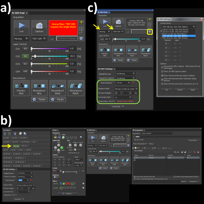
Figure 1. Microscope acquisition settings. (A) Highlights the N-SIM Pad settings used for the experiment and the 'Wrong Fiber' error when the Single channel and Fiber modes are not selected. (B) All windows needed to set-up, record and reconstruct a structured illumination image on the SIM system. (C) N-SIM Pad and N-SIM Settings pop-out window (yellow box) used to select the Grating Setup after physically placing the 488 nm grating into the microscope.
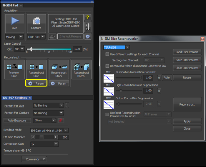
Figure 2. Reconstruction settings for the final image. Upon selecting the 'Param' button (yellow box), select TIRF-SIM from the dropdown menu, and initially set both the 'Illumination Modulation Contrast' (IMC) and 'High Resolution Noise Suppression' (HRNS) to 1.
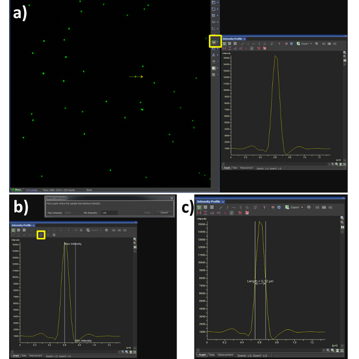
Figure 3. Full Width at Half Maximum (FWHM) measurement. Using the analysis software (A) shows a Gaussian plot from the line intensity tool selected (yellow box) and drawn through a reconstructed SIM image of a bead sample. (B) shows the steps required to quantify the FWHM measurement, by selecting the FWHM button (yellow box) the point of intensity maxima and minima are selected, the output is then obtained (C) showing a resolution of 120 nm in this case. The dip in fluorescence intensity is a known artefact of SIM reconstruction caused by noise, to dampen this effect the high resolution noise suppression can be reduced (Figure 5C), at a cost to resolution.
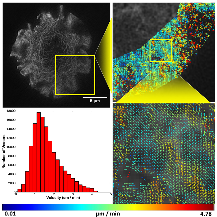
Figure 4. Representative structured illumination data and STICS output. A Jurkat T cell expressing GFP-labelled F-actin imaged using TIRF-SIM on a stimulatory coverslip for immunological synapse generation. Five minutes after contact, a time-course was taken and analyzed using the STICS analysis program. Yellow boxes represent zoomed regions while vector maps demonstrate the retrograde flow of F-actin at the synapse periphery. Vector colors indicate the velocity of the molecular flow in that subregion, velocity data is plotted on a histogram. Due to the z-selectivity of excitation TIRF-SIM provides, the sample can be lost from focus if it detaches or moves away from the coverslip through the time course of the experiment due to ruffling or motility. This is seen here in the top right panel as a reduction in vector density. The reduction is a result of STICS applying the immobile filter to subregions which have shown no fluorescent fluctuations for the period of time set by the user. This result highlights the importance of only selecting regions that contain fluorescence signal for the entire time series.
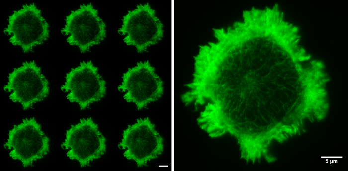
Figure 5. Raw SIM images. The nine raw images on the left show the 9 orientations of the grid pattern needed to produce a TIRF-SIM image. Cell imaged is a Jurkat T cell expressing GFP labelled F-actin, zoomed cell shows one of the nine raw images, demonstrating non-uniform illumination with Moiré fringes, particularly around the cell periphery. Although the structured illumination is not visible the interactions between the illumination and the sample create areas of varying illumination strength, after reconstruction this results in an image with improved resolution. Both scale bars are 5 µm.
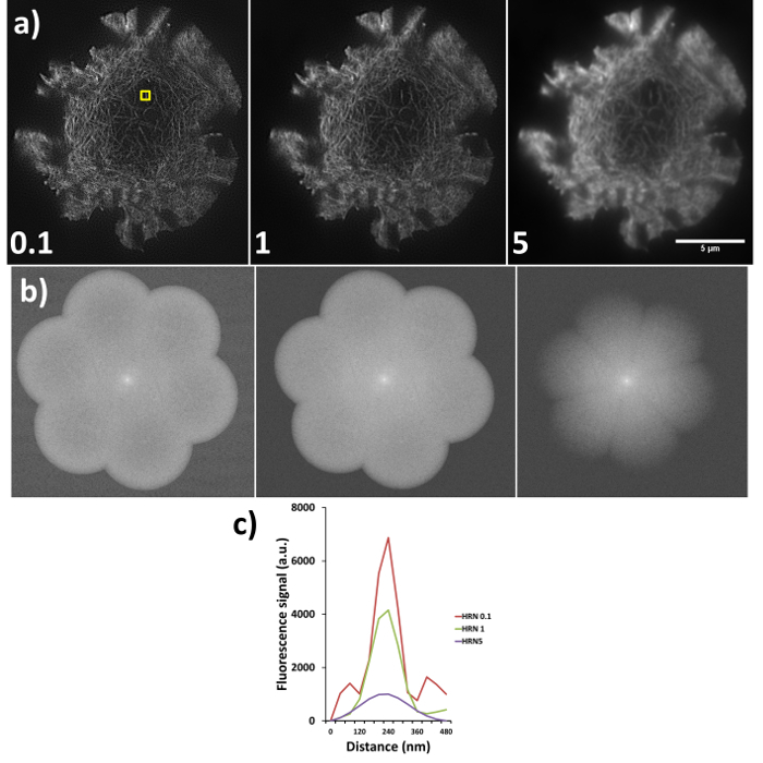
Figure 6. High resolution noise suppression (HRNS) settings. Sub-optimal settings lead to sub-optimal image reconstruction; (A) shows the differences in reconstructed data (settings used shown at bottom left of each image), where lower HRNS leads to increased background noise outside the petal region and higher HRNS can reduce the resolution and result in a loss of the finer details. (B) Represents the forward Fourier transform of images in (A) where peripheral information indicates higher resolution data; note the clipped petals of the transform when HRNS is set to 5, indicating reduced image resolution. (C) demonstrates the full width half maximum (FWHM) of the actin fiber (yellow box in a) at the different settings, FWHM measurements through the software gave reading of 90 nm, 100 nm and 180 nm for HRNS settings of 0.1, 1, and 5 respectively.
Discussion
This technique will allow researchers to image and quantify previously unresolvable details in cells expressing fluorescence. In our results we show that F-actin flows in a symmetrical fashion from the cell periphery towards the cell center in the T cell IS. These findings are consistent with previous results from 1D line profile kymograph data13 and extend the capacity of analysis to 2D and super-resolution data.
The presented technique is a progression from kymograph imaging which is limited to plotting fluorescence intensity fluctuations through a single 1D line over time. In comparison the current technique allows quantification of whole cell molecular flow with both directionality and speed extracted. While speckle imaging has also shown actin dynamics14 within the 2D environment, the speckle technique can be limited by difficulties with correct labeling densities and only visualizes a subpopulation of actin.
The most important steps to achieve these results are to optimize the transfection efficiency of the particular cells being used by the researcher and alignment of the SIM microscope optics and grating pattern. Choosing the correct size of subregion depends on the sample characteristics, and is important as too small a setting will mean faster moving fluorescence is lost by the correlation analysis, but choosing too large a subregion will mean potential loss of nuances in the extra data acquired using super-resolution methods.
Subregion denotes the number of pixels summed to create a super-pixel for velocity mapping analysis, increasing this may improve reliability for tracking faster moving objects. The subregion spacing is the gap between data within superpixels. When the subregion spacing is lower than the subregion size, these adjacent vectors will share some information, increasing this setting could reduce directional consistency of the final vectormap generated. The maximum lag time controls the time correlation analysis, where the number inputted is the maximum number of time lags before analysis ends.
Reconstruction of the final image requires illumination modulation contrast (IMC) and high resolution noise suppression (HRNS) settings to be selected. Optimal settings may differ from sample to sample. IMC helps distinguish the striped illumination pattern on the sample, and reduces reconstruction artefacts. HRNS can reduce artefacts from low contrast data by 'clipping' high resolution data from the Fourier transform; to maintain maximum resolution capabilities and minimize reconstruction artefacts these are normally set at 1.
Limitations of this technique are based around the 2D nature of the process, as the STICS software cannot analyze 3D data the technique is limited to TIRF-SIM or 2D-SIM, this therefore requires the sample to be relatively flat against the coverslip. Another technical disadvantage is that TIRF-SIM requires 9 raw frames to be collected before reconstructing the final super-resolution image, as such with our settings of 50 msec frame acquisitions and the time taken by the SIM microscope to reorient the grid pattern; frame rates of ≈1 sec are achieved. Compared with other super-resolution technique acquisition times and the large field of view these limitations are acceptable for most applications.
The results presented here are comparable with datasets from standard TIRF imaging of F-actin flow in immunological synapse formation. The good agreement between imaging modalities demonstrates STICS is robust against potential SIM reconstruction artefacts and also that the image acquisition settings used during SIM are acceptable for data analysis. By using super-resolution datasets with smaller pixel sizes more data can be extracted from individual cells and dynamics of sub-diffraction cellular micro-domains may be investigated.
After grasping this technique any molecular flow can be imaged and quantified, with scope to non-invasively investigate a multitude of questions regarding flow at the plasma membrane, or when sampling with a confocal microscope, anywhere in the x-y plane of the cell.
Disclosures
The authors declare that they have no competing financial interests.
Acknowledgements
D.M.O. acknowledges European Research Council grant No. 337187 and the Marie-Curie Career Integration Grant No. 334303. P.W.W. acknowledges the Natural Sciences and Engineering Research Council of Canada's Discovery Grant program.
Materials
| Name | Company | Catalog Number | Comments |
| Consumables: | |||
| Jurkat E6.1 cells | APCC | ATTC TIB-152 | |
| RPMI | Life Technologies | 21875-091 | |
| FBS | Sigma | F7524-500ML | |
| Penicillin-Strepromycin | Life Technologies | 15140-122 | |
| HBSS | Life Technologies | 14025-050 | |
| HEPES | Life Technologies | 15630-056 | |
| #1.5 8-well Labtek coverslips | NUNC, Labtek | 155409 | |
| LifeAct GFP construct | Ibidi | 60101 | |
| OptiMem | Life Technologies | 51985-042 | |
| anti-CD3 | Cambridge Bioscience | 317315 | |
| anti-CD28 | BD Bioscience / Insight Biotechnology | 555725 | |
| PBS | Life Technologies | 20012-019 | |
| Lens oil | |||
| Name | Company | Catalog number | Comments |
| Equipment: | |||
| Gene Pulsar Xcell System | BioRad | 165-2660 | |
| Cuvette (0.4cm) | BioRad | 165-2088 | |
| Centrifuge (5810R) | Eppendorf | 5805 000.327 | |
| Centrifuge (Heraeus) | Biofuge pico | 75003235 | |
| 6 well plate | Corning | 3516 | |
| Stage-top incubator | Tokai Hit | INUH-TIZSH | |
| Nikon N-SIM microscope | Nikon | Contact company | |
| Nikon Analyse software | Nikon | Contact company | |
| Incubator (190D) | LEEC | Contact company |
References
- Monks, C., Freiberg, B., Kupfer, H., Sciaky, N., Kupfer, A. Three-dimensional segregation of supramolecular activation clusters in T cells. Nature. 395, 82-86 (1998).
- Lanzavecchia, A. Antigen-specific interaction between T and B cells. Nature. 314, 537-539 (1985).
- Grakoui, A., et al. The immunological synapse: a molecular machine controlling T cell activation. Science.285, (5425), 221-227 (1999).
- Delon, J., Bercovici, N., Liblau, R. Imaging antigen recognition by naive CD4+ T cells: compulsory cytoskeletal alterations for the triggering of an intracellular calcium response. European Journal of Immunology. 28, (2), 716-729 (1998).
- Varma, R., Campi, G., Yokosuka, T., Saito, T., Dustin, M. T Cell Receptor-Proximal Signals Are Sustained in Peripheral Microclusters and Terminated in the Central Supramolecular Activation Cluster. Immunity. 25, (1), 117-127 (2006).
- Rust, M. J., Bates, M., Zhuang, X. Sub-diffraction-limit imaging by stochastic optical reconstruction microscopy (STORM). Nature methods. 3, 793-796 (2006).
- Betzig, E., et al. Imaging intracellular fluorescent proteins at nanometer resolution. Science. 313, (5793), 1642-1645 (2006).
- Klar, T. A., Jakobs, S., Dyba, M., Egner, A., Hell, S. W. Fluorescence microscopy with diffraction resolution barrier broken by stimulated emission. Proceedings of the National Academy of Sciences. 97, (15), 8206-8210 (2000).
- Gustafsson, M. G. Surpassing the lateral resolution limit by a factor of two using structured illumination microscopy. Journal of Microscopy. 198, (2), 82-87 (2000).
- Hebert, B., Costantino, S., Wiseman, P. W. Spatiotemporal image correlation spectroscopy (STICS) theory, verification, and application to protein velocity mapping in living CHO cells. Biophysical Journal. 88, (5), 3601-3614 (2005).
- Ashdown, G. W., Cope, A., Wiseman, P. W., Owen, D. M. Molecular Flow Quantified beyond the Diffraction Limit by Spatiotemporal Image Correlation of Structured Illumination Microscopy Data. Biophysical Journal.107, (9), 21-23 (2014).
- Brown, C. M., et al. Probing the integrin-actin linkage using high-resolution protein velocity mapping. Journal of Cell Science. 19, (24), 5204-5214 (2006).
- Yi, J., Xufeng, S. W., Crites, T., Hammer, J. A. Actin retrograde flow and actomyosin II arc contraction drive receptor cluster dynamics at the immunological synapse in Jurkat T cells. Molecular Biology of the Cell. 23, (5), 834-852 (2012).
- Watanabe, N., Mitchison, T. J. Single-molecule speckle analysis of actin filament turnover in lamellipodia. Science. 8, (5557), 1083-1086 (2002).