×
Total system magnification is found by multiplying the magnification provided by each component in the optical system. Most of the magnification is usually provided by
the objective lens (\(M_{obj}\)), but additional magnification may be introduced at various points in the system.
We broadly classify additional system magnification not provided by the objective lens as either ‘camera relay’ (\(M_{relay}\)) or ‘system magnification’ (\(M_{system}\)). We make this distinction for multiple reasons, including in order
to differentiate whether or not the magnification occurs in the light path between the pinhole disk of a spinning disk confocal microscope and the sample.
‘Camera relay’ (\(M_{relay}\)) applies to magnification that occurs after emission light is collected through the pinholes of a spinning disk. Since this magnification does not occur between the disk and the sample, the back-projected
pinhole size is unaffected. However, the resulting confocal image is still magnified on the detector, affecting the sampling rate on the detector. Usually, ‘camera relay’ magnification occurs between the spinning disk scanner and the
camera in the form of a camera adapter.
‘System magnification’ (\(M_{system}\)) includes magnification by components occurring between the disk and the specimen, which does affect the back-projected pinhole size (important for confocal optical sectioning and resolution
enhancement), just like the objective lens. ‘System magnification’ is often provided by a tube lens (e.g. a 1.5X tube lens instead of the standard 1X), relay optics in the spinning disk confocal system, etc.
The total system magnification, \(M_{tot}\), is found here by multiplying \(M_{obj}\), \(M_{relay}\), and \(M_{system}\) .
\(M_{tot} = M_{obj} * M_{system} * M_{relay}\)(1)
Numerical Aperture, usually abbreviated as 'NA', is how the resolution of a microscope is measured. NA is a dimension-less measure of the range of angles with
which an optical component is able to accept or transmit light, and is described by below, where \(\eta\) is the refractive index of the immersion medium and \(\alpha\) is half the acceptance
angle of the lens.
NA = \(\eta\) sin \( \alpha\) (2)
The microscope objective determines the brightness of illumination, and rises with higher Numerical Aperture (NA) and falls with increasing magnification (\(M_{obj}\)).
Note that the calculation for Brightness is different for transmitted and reflected light imaging as the former requires a seperate condenser
for illumination.
\(Brightness_{dia} = 10^4 * \frac{(NA^2)}{(M_{obj})^2}\) (3)
\(Brightness_{epi} = 10^4 * \frac{(NA^4)}{(M_{obj})^2}\) (4)
Depth of Field (DoField) refers to the maximum Z distance from the most in-focus plane to the furthest plane that can be considered to still be in reasonable focus,
and evaluated at the object plane. This is slightly different from 'Depth of Focus', where this distance is evaluated in the detector plane.
A number of methods have been described for calculating DoField. For this tool, we use the equation described by Young et al.\(^1\) and shown below . The authors provide a straightforward
criterion: two points separated by a certain distance along the z axis can be considered to be in reasonable simultaneous focus if the spherical wavefronts emanating from these points have less than a quarter wavelength difference in
position at the highest angle collected by the objective, evaluated when the middle of those wavefronts overlap at the entrance pupil of the objective lens.
DoField = \(\frac{λ_{ex}}{4\eta(1-\sqrt{1 - (\frac{NA}{\eta})^2})}\) (5)
In order to help avoid confusion with optical sectioning in a confocal microscope, we only provide DoField calculations for widefield imaging scenarios in this tool.
Depth of Focus (DoFocus) is conceptually similar to Depth of Field, but is instead evaluated at the detector plane rather than the object plane. We must account for
the longitudinal (axial) magnification of the optical system, as well as any change in refractive index between the detector medium (\(\eta\) = 1.0) ) and the object immersion medium. This is found using below.
DoFocus = DoField * \(\frac{(M_{tot})^2}{\eta}\) (6)
Lateral resolution refers to the optical resolution in the XY directions and is calculated using the Rayleigh Criterion in this tool.
The Rayleigh Criterion\(^2\) is a generally accepted metric for calculating the resolving power of an optical system. According to the Rayleigh Criterion, the closest possible spacing between two identical point-emitters at which they can
still be considered optically resolved occurs when the point of maximum intensity of one emitter (peak of the Airy disk) overlaps with the first diffraction minimum of the other (first dark ring).
For widefield imaging, the Rayleigh Criterion for lateral resolution, \(r_{lat-WF}\), can be found using , where \(NA_{obj}\) is the numerical aperture of the objective, \(NA_{cond}\) is the
numerical aperture of the condenser, \(λ_{em}\) is the detected wavelength (emission for fluorescence). \(λ_{em}\) is assumed to be 546 nm for diascopic (transmitted light) imaging, corresponding to the center wavelength of light allowed
to pass through a typical green interference filter.
\(r_{lat-WF} = \frac{1.22λ_{em}}{(NA_{obj} + NA_{cond})}\) (7)
For widefield episcopic (reflected light, epifluorescence) imaging, the objective also acts as the condenser. This allows us to simplify to .
\(r_{lat-WF} = \frac{0.61λ_{em}}{NA_{obj}}\) (8)
Axial resolution refers to the optical resolution along the optic (Z) axis, and calculated according to the Rayleigh Criterion\(^3\).
For widefield diascopic (transmitted light) imaging, axial resolution (\(r_{ax-WF}\)) may be calculated using , where \(NA_{obj}\) is the numerical aperture of the objective, \(NA_{cond}\) is
the numerical aperture of the condenser, \(\eta\) is the refractive index of the immersion medium, and \(λ_{em}\) is the detected wavelength (emission for fluorescence). For the purpose of this tool, \(λ_{em}\) is assumed to be 546 nm for
diascopic imaging, corresponding to the center wavelength of light allowed to pass through a typical green interference filter.
\(r_{ax-WF} = \frac{2\etaλ_{em}}{(\frac{NA_{obj} + NA_{cond}}{2})^2}\) (9)
For widefield episcopic (reflected light, epifluorescence) imaging, the objective also acts as the condenser. This allows us to simplify to .
\(r_{ax-WF} = \frac{2\etaλ_{em}}{(NA_{obj})^2}\) (10)
Back-projected pixel size (\(pix_{proj}\)) in a widefield or spinning disk confocal microscope (where an array sensor such as a CMOS or CCD camera is
used) is the apparent size of a single camera pixel when back-projected into the specimen plane, which accounts for the effects of magnification. This value is simply found by dividing the real pixel size, \(pix_{real}\), by the total
magnification of the system, \(M_{tot}\), as described in .
\(pix_{proj} = \frac{pix_{real}}{M_{tot}}\) (11)
Calculating the equivalent back-projected pixel size for a point-scanning confocal microscope, referred to as ‘virtual pixel size’ (\(pix_{virt}\)) here, is described by . The confocal
aperture is the maximum scan area of the instrument at 1X magnification. \(pix_{virt}\) is calculated by dividing the width of the confocal aperture (\(aperture_{conf}\)) by three factors: the number of ‘active pixels’ (the number of
times the signal from the specimen is sampled during a single sweep across the width of the scan area, \(pix_{active}\)), the magnification provided by the objective lens (\(M_{obj}\)), and the 'scan zoom' (the percentage of the width of
the confocal aperture over which the beam is deflected in scanning the sample, \(zoom_{conf}\)).
\(pix_{virt} = \frac{aperture_{conf}}{M_{obj} * {zoom}_{conf} * pix_{active}}\) (12)
Back-projected pinhole radius (BPPR) is the effective de-magnified size of the pinhole aperture(s) back-projected in the specimen plane, and is more
specifically represented by the variables \(BPPR_{point}\) for point-scanning confocal and \(BPPR_{disk}\) for spinning disk confocal.
\(BPPR_{point}\) is found simply by dividing the real pinhole radius, \(r_{pinhole}\), by the objective magnification, \(M_{obj}\) . Note that with standard point-scanning confocal
instruments, users almost never introduce any real optical magnification beyond that provided by the objective lens. This is because additional ‘magnification’ in point-scanning confocal microscopes is almost always best realized using
‘scan zoom’, where the beam is scanned over a smaller portion of the confocal aperture.
\(BPPR_{point} = \frac{r_{pinhole}}{M_{obj}}\) (13)
\(BPPR_{disk} = \frac{r_{pinhole}}{M_{obj} * M_{system}}\) (14)
Back-projected pinhole radius is slightly different to calculate for a spinning disk confocal system , as you do also have to account for additional magnification that may be introduced
between the actual spinning disk and the sample (\(M_{system}\)), in addition to that provided by the objective lens. Unlike point-scanners, this is not uncommon for spinning disk systems. Note that additional magnification provided by
camera adapters located after the spinning disk and before the camera doesn’t affect the back-projected pinhole radius, so is not included in the calculation here (though it is accounted for when considering the sampling rate on the
camera).
The Airy Disk is the 2D (XY) diffraction pattern formed by imaging a point emitter, and has a radius measured as the distance from the central Intensity
maximum to the first diffraction minimum (dark ring), and whose diameter constitutes one Airy Unit (AU). This is an important concept, especially for confocal microscopy, where the pinhole aperture diameter is generally described in terms
of AU. The pinhole aperture is what gives the confocal microscope its optical sectioning ability, and adjustment of its diameter directly modulates both XYZ resolution and optical section thickness. The radius of an Airy Disk,
\(r_{Airy}\), can be calculated using , which you may notice is essentially the same as the widefield Rayleigh lateral resolution from .
\(r_{Airy = \frac{0.61\lambda}{NA_{obj}}}\) (15)
Expressing the pinhole aperture diaphragm opening in terms of Airy Units (AU) is simply performed by finding the ratio of the back-projected pinhole radius (BPPR), which accounts for the effects of magnification, to the radius of the Airy
disk (\(r_{Airy}\)), as shown by below. Please note that you should use \(BPPR_{point}\) for point-scanning systems and \(BPPR_{disk}\) for spinning disk systems in place of BPPR when
calculating the number of Airy units using .
\(AU = \frac{BPPR}{r_{Airy}}\) (16)
The resolution of a confocal microscope is less straightforward to estimate than the typical widefield case, and is a subject that has been
extensively explored. It has been shown that, while the information content of confocal fluorescence images in the spatial frequency domain is theoretically double that of widefield fluorescence images, when considered at practical signal
levels in the spatial domain the improvement is closer to a factor of 1.4 (in XYZ), assuming an infinitely small pinhole aperture\(^{4, 5}\).
A more recent review of the subject\(^5\) provides a detailed evaluation of both resolution and optical sectioning in a confocal microscope, including figures detailing the non-linear responses of lateral (XY) resolution, axial (Z)
resolution, and optical sectioning to pinhole diameter.
For this tool we have estimated fits for both the lateral and axial response curves, where the dependent variable is the scaling factor to be used when calculating resolution and represented by \(C_{lat}\) and \(C_{ax}\) , respectively. We have scaled these curves to match the Rayleigh Criterion instead of full width at half
maximum (FWHM), as originally presented. A \(4^{th}\) order polynomial is used to provide a reasonable estimate of \(C_{lat}\), and a \(6^{th}\) order polynomial for \(C_{ax}\).
\(C_{lat} = -0.2908AU^4 + 0.4884AU^3 - 0.0714AU^2 + 0.0298AU + 0.4357\) (17)
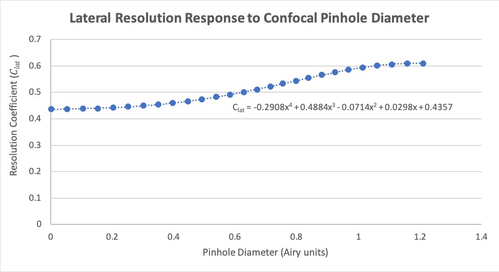 . The relationship between lateral resolution in a confocal microscope and pinhole diameter, normalized to the Rayleigh Criterion for resolution.
\(C_{ax} = -0.0765AU^6 + 0.6359AU^5 - 1.9752AU^4 + 2.7427AU^3 - 1.5335AU^2 + 0.2905AU + 0.7143\) (18)
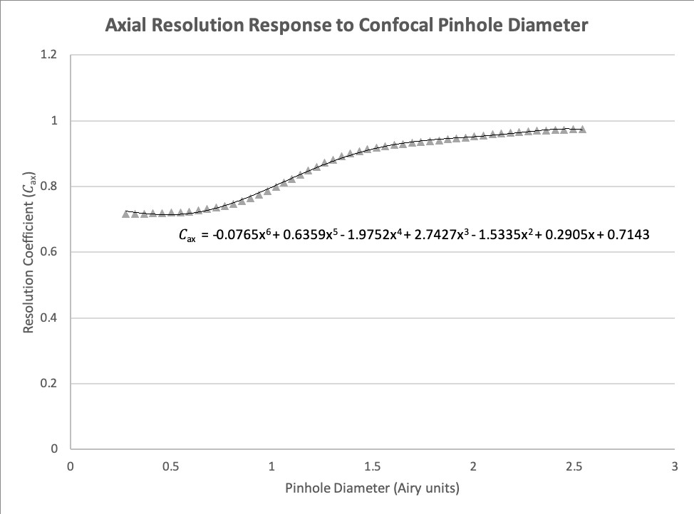 . The relationship between axial resolution in a confocal microscope and pinhole diameter, normalized to the Rayleigh Criterion for resolution.
The Rayleigh lateral resolution limit (\(r_{lat-conf}\)) for a confocal microscope can be estimated using . As the number of AUs approaches 0, the scaling factor \(C_{lat}\) approches its
lower bound value of about 0.436, which represents a 1.4x increase in resolution over the usual coefficient of 0.61, as used in our widefield Rayleigh lateral resolution equation from earlier . 1.2 is chosen as an upper limit because this is where the resolution response curve levels off, approaching a value of 0.61 and above which we clamp the scaling factor at 0.61 .
The only difference from the widefield Rayleigh limit equation is that we use excitation wavelength instead of emission for our confocal resolution measurements.
\(r_{lat-conf} = \begin{cases}
\frac{C_{lat}\lambda_{ex}}{NA_{obj}}, & 0\le AU\le 1.2 \\
\frac{0.61\lambda_{ex}}{NA_{obj}}, & 1.2\lt AU
\end{cases}\) (19)
The axial resolution limit \(r_{ax-conf}\) for a confocal microscope can be estimated using where it is calculated using different functions if AU is less than 0.35, between 0.35 and 2.5, and
more than 2.5. From 0 to 0.35 AU the scaling factor is clamped at 1.43, representing a 1.4x increase in resolution over the scaling factor of 2 used when calculating widefield axial resolution. Above 2.5 AU the axial response curve levels
off, so we clamped the scaling factor to 2, as used for the widefield Rayleigh axial resolution .
\(r_{ax-conf} = \begin{cases}
\frac{1.43\eta\lambda_{ex}}{(NA_{obj})^2}, & AU\le 0.3 \\
\frac{2{\eta}C_{ax}\lambda_{ex}}{(NA_{obj})^2}, & 0.3\lt AU\lt 2.5 \\
\frac{2\eta\lambda_{ex}}{(NA_{obj})^2}, & 2.5\le AU
\end{cases}\) (20)
Please note that the confocal resolution equations described in this section are simple estimates for best-case imaging scenarios, and should not be interpreted as complete analytical solutions. In reality, confounding factors such as low
signal-to-noise (especially with narrow pinholes) and optical aberrations limit the practical performance you can expect.
Confocal optical sectioning is calculated using an equation previously described\(^5\), where optical sectioning is considered in terms of
contrast transfer with increasing defocus, accounting for the effect of the pinhole in blocking out-of-focus light. As with axial resolution, we scale a version of their equation to coincide with the Rayleigh limit instead of full width
at half maximum (FWHM) in order to estimate optical sectioning (\(\Delta z_{conf}\), , Figure 3). This equation only fits the response up to a pinhole diameter of 3 AU, above which optical
section thickness is not provided.
\(\Delta z_{conf} = \begin{cases}
\frac{1.5\eta\lambda_{ex}}{(NA_{obj})^2}\sqrt[3]{1+1.47AU^3}, & 0\le AU\le3
\end{cases}\) (21)
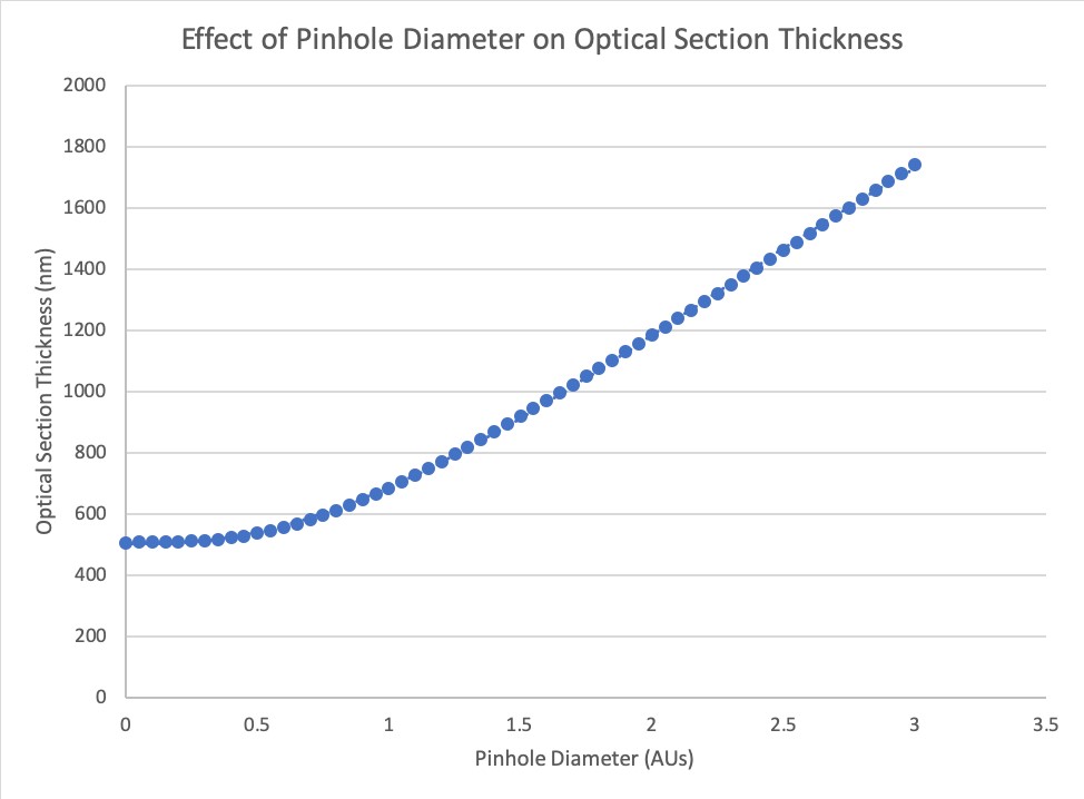 . The relationship between optical sectioning in a confocal microscope and pinhole diameter, measured in Airy Units (AU). For this example, we are assumming an excitation wavelength
\(\lambda_{ex}\) of 500 nm, \(\eta\) = 1.5 and NA = 1.49.
. The relationship between optical sectioning in a confocal microscope and pinhole diameter, measured in Airy Units (AU). For this example, we are assumming an excitation wavelength
\(\lambda_{ex}\) of 500 nm, \(\eta\) = 1.5 and NA = 1.49.
This term originated in the field of signal processing and is formalized by the Nyquist-Shannon Sampling Criterion\(^6\), which states that in order for a given
frequency (single sine wave) to be reconstructed, it must be sampled at least twice. For example, in the realm of digital imaging, this means that if the calculated optical resolution is 200 nm, then the pixel size must be 100 nm or
smaller in order to properly sample the finest details. In practice, a sampling rate of 2.3 – 4X is a more commonly recommended range for high resolution imaging.
The sampling rate is calculated in one of three ways, depending on whether or not it's a widefield (\(f_{WF}\), ), spinning disk confocal (\(f_{conf-disk}\), ), or point-scanning confocal (\(f_{conf-point}\), ) instrument.
\(f_{WF} = \frac{r_{lat-WF}}{pix_{proj}}\) (22)
\(f_{conf-disk} = \frac{r_{lat-conf}}{pix_{proj}}\) (23)
\(f_{conf-point} = \frac{r_{lat-conf}}{pix_{virt}}\) (24)
For the widefield case, it is equal to the widefield lateral resolution (\(r_{lat-WF}\)) divided by the back-projected pixel size (\(pix_{proj}\)) of the camera. For the spinning disk case, it is the confocal lateral resolution
(\(r_{lat-conf}\)) divided by \(pix_{proj}\), since this technique also used a camera as a detector. For point-scanning, it is (\(r_{lat-conf}\)) divided by the virtual pixel size (\(pix_{virt}\)) since a single pixel detector is used and
the illumination spot is scanned.
- Young, I.T. et al. Depth-of-Focus in Microscopy. SCIA’93, Proc. of the 8th Scandinavian Conference on Image Analysis, Tromso, Norway, 493-498 (1993).
-
Lord Rayleigh, F.R.S. Investigations in Optics, with special reference to the Spectroscope. Phil. Mag. 8, 261 – 274 (1879).
-
Oldenbourg, R. and Shribak, M. Microscopes. In M. Bass (Ed.). Handbook of Optics, Volume 1: Geometrical and Physical Optics, Polarized Light, Components and Instruments (28.1-28.62). U.S.A.: McGraw Hill.
-
Wilson, T. Optical sectioning in confocal fluorescent microscopes. J. Micr. 154, 143 – 156 (1989).
-
Wilson, T. Resolution and optical sectioning in the confocal microscope. J. Micr. 244, 113 – 121 (2011).
-
Shannon, C. E. Communication in the Presence of Noise. Proceedings of the IRE, 37, 10–21 (1949).